The Lorenz System

The Lorenz system was the first dynamical system known for exhibiting chaotic behavior. It was developed as a simplified model for describing atmospheric convection (E N Lorenz 1963). The dynamical system consists of three variables, denoted \(x, y, z\), obeying the equations:

(45)\[\begin{align} \dot{x} &= \sigma (y - x) \\ \dot{y} &= x ( \rho - z) - y \\ \dot{z} &= x y - \beta z \end{align}\]

These variables roughly represent the convection rate and the horizontal and vertical temperature variation in a fluid layer. There are three parameters, \(\sigma, \rho, \beta\), representing the Prandtl number, the Rayleigh number, and the relative dimension of the fluid. These dynamical equations are now known as the “Lorenz equations”.

The Lorenz system is the classic example of “deterministic chaos”. In Lorenz’s own words, such chaos happens “when the present determines the future, but the approximate present does not approximately determine the future.” In other words, the dynamics of the system is deterministic, as it is the solution to a set of differential equations, whose solutions are uniquely determined by initial conditions. However, the solution is very sensitive to the initial condition, such that tiny changes in the initial values would lead to dramatic differences in the long term.

To examine such unusual behavior, we will numerically solve the Lorenz equations.

import numpy as np
import scipy.integrate as intgr
import matplotlib.pyplot as plt

def lorenz(xyz, t, sigma, rho, beta):
    """
    Lorenz equations, with parameters as arguments.
    """
    x, y, z = xyz    # parse variables
    dxdt = sigma * (y - x)
    dydt = x * (rho - z) - y
    dzdt = x * y - beta * z
    return [dxdt, dydt, dzdt]

Steady states and stability

The steady states of the Lorenz system can be found analytically. If we set the right-hand side of the equations to zero, the solutions will be:

(46)\[\begin{equation} x^* = y^* = z^* = 0, \quad \textrm{or} \quad x^* = y^* = \pm \sqrt{\beta (\rho - 1)} \;\;\&\;\; z^* = \rho - 1. \end{equation}\]

There is a trivial solution at the origin, and a pair of solutions that are located on the same constant \(z\) plane and symmetrical about the \(z\) axis.

If the parameter \(\rho < 1\), the two nontrivial solutions would not exist because of the squareroot. In this case, we may expect that the only steady state at the origin is stable. Let us verify this by solving the equations from some random initial values.

sigma = 10.
beta = 8/3.
rho = 0.5

T = 10.    # total time to run
dt = 0.01    # time step
time_points = np.arange(0., T, dt)

repeat = 10    # number of trajectories to plot
sol0_list = []

for r in range(repeat):
    init = np.random.rand(3)*2-1
    sol0 = intgr.odeint(lorenz, init, time_points, args=(sigma, rho, beta))
    sol0_list.append(sol0)

These solutions represent trajectories in the 3-d (x,y,z) space. To visualize them, we can plot the projection of these trajectories in the (x,z) plane.

plt.figure()
for r in range(repeat):
    sol0 = sol0_list[r]
    plt.plot(sol0[:,0], sol0[:,2])    # plot trajectories projected onto the (x,z) plane
    plt.plot([sol0[0,0]], [sol0[0,2]], 'b^')    # blue trianble labels starting point of each trajectory
plt.plot([0], [0], 'rx')    # steady state at the origin
plt.xlabel(r'$x$')
plt.ylabel(r'$z$')
plt.show()

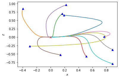
It can be seen that all trajectories do converge to the origin.

When \(\rho\) is larger than \(1\), the pair of nontrivial steady states appear, and the steady state at the origin is no longer stable. Let us visualize this situation.

sigma = 10.
beta = 8/3.
rho = 2.

T = 10.    # total time to run
dt = 0.01    # time step
time_points = np.arange(0., T, dt)

repeat = 10    # number of trajectories to plot
sol1_list = []

for r in range(repeat):
    init = np.random.rand(3)*2-1
    sol1 = intgr.odeint(lorenz, init, time_points, args=(sigma, rho, beta))
    sol1_list.append(sol1)

x1 = y1 = np.sqrt(beta*(rho-1))    # nontrivial steady state
z1 = rho-1

plt.figure()
for r in range(repeat):
    sol1 = sol1_list[r]
    plt.plot(sol1[:,0], sol1[:,2])    # plot x as a function of time
    plt.plot([sol1[0,0]], [sol1[0,2]], 'b^')    # blue trianble labels starting point of each trajectory
plt.plot([x1], [z1], 'rx')    # steady state at the origin
plt.plot([-x1], [z1], 'rx')    # steady state at the origin
plt.xlabel(r'$x$')
plt.ylabel(r'$z$')
plt.show()

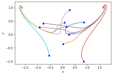
We see that the system is bistable: the trajectories flow to one of the two nontrivial steady states depending on the initial values.

However, this is not the whole story. When the value of \(\rho\) becomes sufficiently large, the two steady states also become unstable, and the system becomes “chaotic”. We will explore this situation below.

Irregular oscillation and strange attractor

Lorenz first observed this strange behavior when he used the parameter values \(\sigma = 10\), \(\beta = 8/3\), and \(\rho = 28\). Let us reproduce his observations.

sigma = 10.
beta = 8/3.
rho = 28.

T = 50.    # total time to run
dt = 0.01    # time step
time_points = np.arange(0., T, dt)

repeat = 10    # number of trajectories to plot
sol2_list = []

for r in range(repeat):
    init = np.random.rand(3)*2-1
    sol2 = intgr.odeint(lorenz, init, time_points, args=(sigma, rho, beta))
    sol2_list.append(sol2)

The first strange feature of the solution that Lorenz noticed was an irregular oscillation. To see this, let us plot one of the variables, like \(x\), as a function of time. We will show just one of the solutions.

x2 = y2 = np.sqrt(beta*(rho-1))    # nontrivial steady state
z2 = rho-1

plt.figure()
# plt.axhline(0, color='k', lw=1)    # steady state at the origin
plt.axhline(x2, color='k', lw=1)    # one of the nontrivial steady states
plt.axhline(-x2, color='k', lw=1)    # the other nontrivial steady state
plt.plot(time_points, sol2[:,0])    # plot x as a function of time
plt.xlabel(r'$t$')
plt.ylabel(r'$x$')
plt.show()

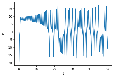
It looks like the solution oscillates around one unstable steady state for a number of times, then switches to oscillating around the other one. However, the behavior is aperiodic, as we can see that the number of times it goes around each steady state varies with time, in an apparently random fashion.

We can also visualize the solution as a trajectory projected onto the (x,z) plane.

plt.figure()
plt.plot(sol2[:,0], sol2[:,2])    # plot trajectories projected onto the (x,z) plane
plt.plot([sol2[0,0]], [sol2[0,2]], 'b^')    # blue trianble labels starting point of each trajectory
plt.plot([x2], [z2], 'rx')    # steady state
plt.plot([-x2], [z2], 'rx')    # steady state
plt.xlabel(r'$x$')
plt.ylabel(r'$z$')
plt.show()

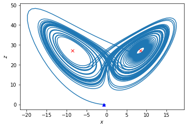
The trajectory seems to circle around each steady state many times, filling out a region that looks like a butterfly.

Let us now visualize all the solutions as trajectories in a 3-d plot (you may turn on the interactive mode, so that you can rotate the plot to see from different angles).

from mpl_toolkits.mplot3d import Axes3D
# uncomment the following line to turn on interactive mode
# %matplotlib widget

fig = plt.figure()
ax = fig.add_subplot(projection='3d')
for r in range(repeat):
    sol2 = sol2_list[r]
    ax.plot(sol2[:,0], sol2[:,1], sol2[:,2])
ax.set_xlabel(r'$x$')
ax.set_ylabel(r'$y$')
ax.set_zlabel(r'$z$')
plt.show()

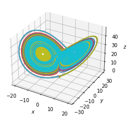
It can be seen that, although the trajectories never stop at any steady state, they are confined to a finite region that looks like two thin disks joined together at an angle. The center of each disk is one of the unstable steady states. Each trajectory circles around on one disk for a certain number of times, and then moves onto the other disk and repeats. The structure formed by the two disks is an “attractor” in the sense that all trajectories starting from any initial values will eventually converge to the same finite region and exhibit the same aperiodic behavior. This structure is quite befittingly called a “strange attractor”. To mark its strangeness, it is mathematically shown to have a fractal dimension of 2.05 (a little “thicker” than 2D disks)!

Sensitivity to initial conditions

Another important feature of the chaotic dynamics is the extreme sensitivity to the initial condition. This is sometimes referred to as the “butterfly effect”, perhaps inspired by the butterfly-looking trajectory in the Lorenz system. It says that a butterfly flapping wings in one place could cause a tornado later in another place faraway, which is a metaphor for the chaotic nature of weather systems. We will examine such sensitivity below.

Let us add a small perturbation to the previous solution at a given time, then solve the equations onward with these perturbed initial values. We will add the perturbation when the solution has settled onto the strange attractor, say at \(t = 20\).

t1 = 20.    # time to add perturbation
init0 = sol2[int(t1/dt)].copy()    # value of original solution at given time
init1 = init0 + 1e-6    # add very small perturbation
time_points1 = np.arange(0., T - t1, dt)
sol3 = intgr.odeint(lorenz, init1, time_points1, args=(sigma, rho, beta))

Let us plot the two solutions side by side to see how they differ.

plt.figure()
plt.axhline(x2, color='k', lw=1)
plt.axhline(-x2, color='k', lw=1)
plt.axvline(t1, color='r', lw=1, label='perturbation')
plt.plot(time_points, sol2[:,0])    # original solution
plt.plot(time_points1 + t1, sol3[:,0])    # perturbed solution
plt.xlabel(r'$t$')
plt.ylabel(r'$x$')
plt.legend(loc='lower left')
plt.show()

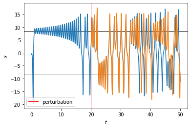
We see that the solutions started very close to each other after the perturbation, as one would expect. However, deviations began to be visible around \(t = 35\), and then the trajectories quickly diverged from each other. In fact, later there were times when one trajectory was going around one steady state, while the other trajectory was going around the other, i.e., being as far from each other as possible within the strange attractor.

Let us examine how fast the solutions diverge by plotting their difference as a function of time.

diff = sol2[int(t1/dt):] - sol3    # difference between solutions, 3d vector
diff = np.sqrt(np.sum(diff**2, axis=1))    # magnitude of difference

plt.figure()
plt.plot(time_points1 + t1, diff)
plt.yscale('log')
plt.ylim(5e-7, 2e3)
plt.xlabel(r'$t$')
plt.ylabel(r'$|\Delta x|$')
plt.show()

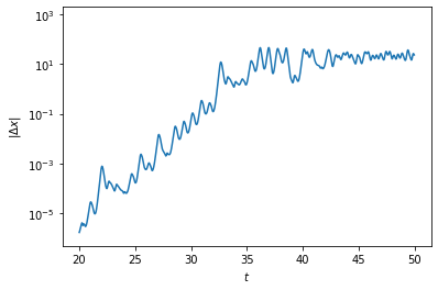
We see that there is a roughly linear increase in the log plot, which eventually flatten out because the difference is bounded by the length scale between the steady states. If we fit the increasing part to a line, we can find the rate of divergence of the solutions, which is the so-called “Lyapunov exponent” of the chaotic system.

slope, intercept = np.polyfit(t1+time_points1[:1500], np.log(diff[:1500]), 1)    # fit line
t_array = time_points1 + t1
d_array = np.exp(np.polyval((slope, intercept), t_array))    # calculate line

plt.figure()
plt.plot(time_points1 + t1, diff)
plt.plot(t_array, d_array, '--', label=f'Lyapunov exponent = {slope:.1f}')
plt.yscale('log')
plt.ylim(5e-7, 2e3)
plt.xlabel(r'$t$')
plt.ylabel(r'$|\Delta x|$')
plt.legend()
plt.show()

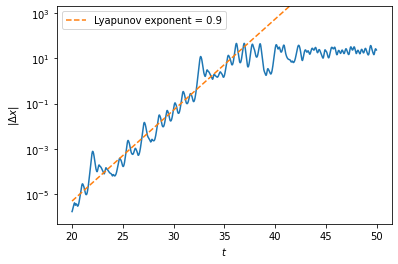
The inverse of the Lyapunov exponent sets a timescale over which small errors in the initial values are amplified to render predictions of the future unreliable. For example, this “Lyapunov time” for typical weather models is on the order of 10 days, which means weather forecasts are inevitably inaccurate beyond a week or so.

Orbit diagram and bifurcation

Finally, let us study how the behavior of the solution depends on the parameters. It turns out that the chaotic behavior is exhibited when \(\rho > \rho_H \equiv \sigma (\sigma + \beta + 3) / (\sigma - \beta - 1)\). On the other hand, when \(\rho < \rho_P \equiv 1\), the origin is the unique stable steady state. In between \(\rho_P < \rho < \rho_H\), the origin is unstable but the other two steady states \((\pm \sqrt{\beta (\rho - 1)}, \pm \sqrt{\beta (\rho - 1)}, \rho - 1)\) are, so the system is bistable. The location of the steady states and the behavior of the solutions in general can be represented by an orbit diagram shown below. To make this diagram, we vary the value of \(\rho\), and for each \(\rho\) value, we solve the equations from random initial values; then we plot the position of the trajectory at every time point (after some initial period by which the solution has settled down).

sigma = 10.
beta = 8/3.

T = 100.
dt = 0.01
time_points = np.arange(0., 50., 0.01)

rho_list = np.geomspace(0.1, 1000., 401)    # list of rho values geometrically spaced
sol_list = []    # list of solutions of Lorenz equations

for rho in rho_list:
    init = np.random.rand(3)*2-1    # random initial values
    sol = intgr.odeint(lorenz, init, time_points, args=(sigma, rho, beta))
    sol_list.append(sol)

rP = 1    # onset of instability at the origin, pitchfork bifurcation
rH = sigma * (sigma + beta + 3) / (sigma - beta - 1)    # onset of chaos, Hopf bifurcation

plt.figure(figsize=(8,6))
plt.axvline(rP, lw=1, ls=':', label=r'$\rho = 1$')
plt.axvline(rH, lw=1, ls='--', label=r'$\rho = %.3f$' % rH)
plt.axvline(28, lw=1, ls='-', label=r'$\rho = 28$')
for i in range(len(rho_list)):
    rho = rho_list[i]
    sol = sol_list[i]
    y = sol[int(t1/dt):,0]
    x = [rho] * len(y)
    plt.scatter(x, y, s=0.1, c='k', marker='.', edgecolor='none')
plt.xscale('log')
plt.xlabel(r'$\rho$')
plt.ylabel(r'$x$')
plt.legend()
plt.show()

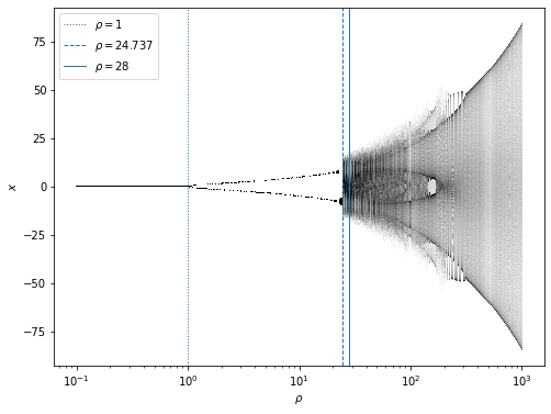
It can be seen that the stable steady state at the origin “bifurcates” into two steady states at \(\rho = 1\). (This is known as the “pitchfork bifurcation” where one fixed point splits into two.) Then at \(\rho_H \approx 24.737\) the two steady states undergo another type of “bifurcation” (known as the “Hopf bifurcation” where a fixed point becomes a saddle point) that leads to the onset of chaos.