Eigenworms
Contents
Eigenworms#
In this notebook, we will use “dimensionality reduction” methods to study animal behavior. As one can imagine, behavior can be highly complex. In some animals, biologists have classified behavior by stereotypical postures or movements that they have defined based on experience. Recent technology, such as high-resolution and high-speed digital camera, has allowed us to take a more quantitative approach by collecting and analyzing behavioral data. However, the data will most likely be high dimensional, as they may represent the shape and position of each body part. Our goal is to see if we can simplify such high-dimensional representation to a much lower dimensional description, and perhaps these “principal” dimensions would match the stereotypical behaviors that were found “manually”. Thus, we look for an automatic and unbiased way of reducing the dimensionality of the data to help us extract the basic modes of behavior.
Our example here is the crawling behavior of the roundworm, C. elegans. In the experiment of (Stephens et al., 2008), the worms were left on a plate to crawl around, and their motion was recorded from the top by a microscope and digital camera at 4 frames per second. A typical image looks like this:


On the right is the processed image where the background has been removed.
The image is 640x480 pixels, but we certainly should not need 307200 variables to describe the posture of the worm in this single frame. In fact, since the body shape of the worm is rather simple — a round tube of rather constant width — we may draw a center curve along the body to represent its shape in each frame. This curve can be described by an array of x and y coordinates for the points along the line. For example, we can divide the curve into 101 segments of equal length, then we can use the coordinates of the 102 endpoints to describe the curve. That amounts to 102 x 2 = 204 variables, a dramatic reduction from the number of pixels. Yet, we can still do a little better by noticing that the shape of the curve does not change if we rotate the whole image. That means we should use the relative positions of the points with respect to each other, not the absolute positions in the image. This can be done by using the angles of the segments as our variables, instead of the x-y coordinates of the endpoints. With that, we are down to 100 variables that can describe the shape of the worm in each frame. This procedure is illustrated in the figure below:

It has been a huge reduction of data dimensionality, from seemingly 307200 to 100. But we have chosen the number 100 just so that it is large enough for constructing a smooth curve. It does not mean that our data is really 100 dimensional. In fact, using dimensionality reduction methods, we will show that the intrinsic dimensionality of the worm shape is even much lower — just about 4 dimensions. (Our final results will not depend on the choice of 100 here, as long as it is large enough to resolve the curve.) We will achieve this final dimensionality reduction by using “principal component analysis” (PCA) below.
Principal Component Analysis#
We start from a processed dataset containing 6655 frames, each represented by a 100 dimensional vector. Thus, we have a 2d-array of shape (6655,100), where each row is one frame. Let us load the data first.
import numpy as np
import matplotlib.pyplot as plt
import matplotlib.animation as anim
data = np.loadtxt('data/wormshapes.csv', delimiter=',')
N = data.shape[0]    # number of data points
D = data.shape[1]    # number of dimensions
print(f'number of data points = {N}, dimension = {D}')
number of data points = 6655, dimension = 100
We can think of each data point as a point in a \(D\)-dimensional space, and we have \(N\) such points in that space. The idea of dimensionality reduction is that maybe these points lie on a lower dimensional subspace, like a 2d plane in a 3d space. In order to find such a subspace, we need to see how much the points vary in each direction. For example, if all points lie on a plane, then there will be variations parallel to the plane but no variation in the perpendicular direction. To find such major directions of variation, we will calculate the covariance matrix of these points.
Let the data be denoted by \(X_{ni}\), where \(n = 1, \cdots, N\) are the indices of the data points and \(i = 1, \cdots, D\) are the indices of the components. The covariance matrix is given by:
where \(\bar{X}_i\) is the mean values of all data points given by:
The covariance matrix is a \((D \times D)\) matrix, whose diagonal elements are the variance of the data points along each axis, and the off-diagonal elements are the covariance between two components.
We can calculate the covariance matrix as follows.
x_mean = np.mean(data, axis=0)    # mean over data points
x_cent = data - x_mean    # centered data
cov = np.dot(x_cent.T, x_cent) / N    # covariance matrix
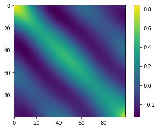
We can visualize the covariance matrix using a heatmap.
plt.figure()
plt.imshow(cov)
plt.colorbar()
plt.show()

There is clear structure in the covariance matrix, which suggests that the data points have larger variation in certain directions than others. However, the largest variations may not be as simple as being along some basis axes of the \(D\)-dimensional space. Rather, we have the freedom to rotate the axes and find the directions of most variation. This can be done by finding the eigenvectors of the covariance matrix that have the largest eigenvalues. We can calculate the eigenvalues and eigenvectors using the numpy.linalg.eig function. (Note that, because the covariance matrix is real and symmetric, all eigenvalues and eigenvectors are real. This allows us to use the eigh function instead.)
w, v = np.linalg.eigh(cov)    # find eigenvalues and eigenvectors of a real symmetric matrix

sort = np.argsort(w)[::-1]    # sort eigenvalues from largest to smallest
w = w[sort]
v = v[:,sort]    # sort eigenvectors accordingly
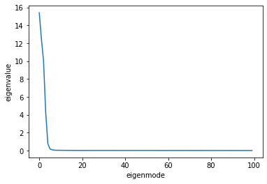
If we plot the sorted eigenvalues, we will see that their values fall off rapidly after the first few modes.
plt.figure()
plt.plot(w)
plt.xlabel('eigenmode')
plt.ylabel('eigenvalue')
plt.show()

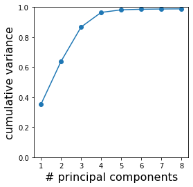
This prompts us to keep only the first few modes, or “principal components” (PC). To help us decide how many principal components we need to keep, we normalize the eigenvalues by their sum. The normalized eigenvalues represent the fraction of the total variance in the data that is captured by each mode. Let us plot the cumulative sum of these fractions to see how much variance is captured by the first few components.
w = w / np.sum(w)    # normalized eigenvalues = variance along each principal component
wsum = np.cumsum(w)    # cumulative sum of normalized eigenvalues = variance captured

plt.figure(figsize=(4,4))
plt.plot(np.arange(1,9), wsum[:8], 'o-')
plt.ylim(0, 1)
plt.xticks(np.arange(1,9))
plt.xlabel('# principal components', fontsize=16)
plt.ylabel('cumulative variance', fontsize=16)
plt.show()

Apparently, the first 4 principal components already capture >96% of the variance present in the data. It means that we can safely ignore the rest of the eigenmodes without sacrificing much accuracy of our description of the data. Therefore, we can use these 4 principal components to form a reduced description of the worm shapes — from 100 to 4 dimensions! (The choice of 4 here is also not unique; depending on the use of the data, we may be satisfied with less if we do not require high accuracy, or we may take a few more if we need more details.)
Let us plot these 4 principal components. They are represented by the corresponding eigenvectors (already normalized by default).
K = 4    # number of principal components to use
PC = v[:,:K]    # eigenvectors for these PCs; each column is one PC

fig, ax = plt.subplots(1,K, figsize=(5*K,4))
for i in range(K):
    ax[i].plot(PC[:,i])
    ax[i].set_title(f'PC{i+1}')
plt.show()

Remember that these are vectors in a 100-dimensional space of the angles of consecutive segments along the worm body. We can use them as new basis vectors to decompose any shape of the worm (represented by a 100-dimensional vector of angles) into components. That is, the shape of the worm can be described by a linear combination of these “eigenworms”.
To visualize the shape of these eigenworms, we need to convert from angles of consecutive segments back to positions of the endpoints. This is done by the following function.
def angle2pos(angles):
    """
    convert from angles of consecutive segments of unit length to positions of their endpoints.
    inputs:
    angles: 1-d array, angles of consecutive segments.
    outputs:
    pos: 2-d array, each row is (x,y) coordinates of an endpoint, centered at zeros.
    """
    dx = np.cos(angles)
    dy = np.sin(angles)
    xsum = np.cumsum(dx)
    ysum = np.cumsum(dy)
    pos = np.zeros((D+1, 2))
    pos[1:,0] = xsum
    pos[1:,1] = ysum
    mean = np.mean(pos, axis=0)
    pos = pos - mean
    return pos
We can now plot the eigenworms. To see appreciable shapes, we will multiply each mode by an amplitude, set to 5.
pos_all = []
for i in range(K):
    pos = angle2pos(PC[:,i]*5)    # convert PC (with amplitude 5) to positions
    pos_all.append(pos)

fig, ax = plt.subplots(1,K, figsize=(5*K,4))
for i in range(K):
    pos = pos_all[i]
    ax[i].plot(pos[:,0], pos[:,1], '.-')
    ax[i].set_aspect('equal')
    ax[i].axis('off')
plt.show()

Reconstructing data#
The ultimate test of our dimensionality reduction is to see if we can recover the original shapes of the worm using only those principal components. In other words, we will try to reconstruct the data from only the projections onto the principal components. Let the principal components be denoted by a matrix \(v_{ik}\), where each column \(k\) represents the \(k\)-th principal component. Then the projections of the original data are given by
We can reconstruct the data from these projections using
Note that here the sum is only over the first \(K\) components. If we had summed over all components (\(k = 1, \cdots, D\)), then we should fully recover the original data, because in that case we simply did a coordinate transformation without any reduction of dimensions. Therefore, the dimensionality reduction that we have achieved is from \(D\) to \(K\) dimensions.
Let us calculate the projected data onto the principal components and the reconstructed data from those projections.
x_project = np.dot(x_cent, PC)    # project (centered) data onto principal components
x_reconstruct = np.dot(x_project, PC.T) + x_mean    # reconstruct data from the projections
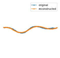
We can plot the original and the reconstructed shape of a worm on top of each other.
pos_original = angle2pos(data[0,:])    # original data from one frame
pos_reconstruct = angle2pos(x_reconstruct[0,:])    # reconstructed data

plt.figure(figsize=(4,4))
plt.plot(pos_original[:,0], pos_original[:,1], '.-', label='original')
plt.plot(pos_reconstruct[:,0], pos_reconstruct[:,1], '.-', label='reconstructed')
plt.xlim(-50, 50)
plt.ylim(-50, 50)
plt.legend()
plt.axis('off')
plt.show()

It looks like our reconstruction is very faithful to the original shape. The small discrepancies are due to our ignoring the “higher order” modes in the decomposition. Nevertheless, the reduced description is much more concise (and space-saving and fast-to-process on computers), and hopefully accurate enough for further studies on the worm behavior (as Stephens et al. show in their research paper; they also show that these principal components have intuitive biological interpretations).
To have a bit more fun, we can make a video of the worm’s movements using both the original and reconstructed data.
plt.rcParams["animation.html"] = "jshtml"
fig, ax = plt.subplots(figsize=(4,4))
ax.set_xlim(-50, 50)
ax.set_ylim(-50, 50)
ax.axis('off')
p0, = ax.plot([], [], '.')
p1, = ax.plot([], [], '.')

def animate(t):
    pos_original = angle2pos(data[t,:])
    pos_reconstruct = angle2pos(x_reconstruct[t,:])
    p0.set_data(pos_original[:,0], pos_original[:,1])
    p1.set_data(pos_reconstruct[:,0], pos_reconstruct[:,1])

mov = anim.FuncAnimation(fig, animate, frames=range(27,87), interval=250)
# mov.save('figures/eigenworms.mp4', fps=4, extra_args=['-vcodec', 'libx264'])
plt.close()
mov

