Multi-layer Perceptron
Contents
Multi-layer Perceptron#
A multi-layer perceptron is a multi-layer feed-forward network. It can be thought of as several simple perceptrons stacked together, with the output layer of one being the input layer of the next. Thus, a \(L\)-layer perceptron has one input layer (the 0th layer), \((L-1)\) hidden layers (the 1st to \((L-1)\)th layers), and one output layer (the \(L\)th layer). There are \(L\) sets of connections, the \(l\)th connection being between the \((l-1)\)th layer and the \(l\)th layer (for \(1 \leq l \leq L\)).
Suppose each layer has \(N_l\) units, \(0 \leq l \leq L\). Let us denote the values of the \(l\)th layer units by \(R^l_i\) for \(i = 1, \cdots, N_l\). Also, let the connection matrix between the \((l-1)\)th and \(l\)th layer be \(W^l_{ij}\), \(1 \leq l \leq L\). The values of the units in each layer is determined by the values of the units in the previous layer according to the equation:
Here \(g(x)\) is a nonlinear activation function, such as \(\operatorname{sgn}(x)\). Note that we set \(R^0_i \equiv S_i\), where \(S_i\) is the input to the network. The output of the final layer, \(R^L_i\), will be the output of the network.
The presence of the hidden layers allows the network to perform much more complex tasks. For example, we have learned that a simple perceptron without hidden layers cannot classify points correctly if they are not linearly separable. However, we will show that a 2-layer perceptron with a sufficiently large hidden layer can perform such classification.
import numpy as np
import matplotlib.pyplot as plt
Multi-layer feed-forward network#
Let us first write a python class to implement a basic multi-layer feed-forward network.
from networks import FeedforwardNetwork, SimplePerceptron
class MultilayerNetwork:
    """
    base class of multi-layer network, each layer is a FeedforwardNetwork.
    """

    def __init__(self, N_list, input_layer=None, connection_list=None, activation='threshold'):
        """
        declare internal variables.
        inputs:
        N_list: list of int, numbers of units in every layer.
        input_layer: 1-d array, input units; can also be pointer to array.
        connection_list: list of 2-d arrays, connection matrices between every consecutive layers.
        activation: 'threshold'|'linear'|other, activation function, can be user-supplied.
        """
        self.N_list = np.asarray(N_list)
        self.L = len(N_list) - 1    # number of layers (excluding input layer)
        if input_layer is None:
            self.input = np.zeros(N_list[0])    # first layer is input
        else:
            self.input = input_layer
        layer = FeedforwardNetwork(N_list[0], N_list[1], activation=activation)    # first layer
        layer.set_network(input=self.input)    # input = network input
        self.layers = [layer]    # list of layers (excluding input layer)
        for l in range(1,self.L):
            layer = FeedforwardNetwork(N_list[l], N_list[l+1], activation=activation)    # new layer
            layer.set_network(input=self.layers[l-1].output)    # input = previous layer's output
            self.layers.append(layer)    # add layer to network
        for l in range(self.L):
            if connection_list is None:
                rand = np.random.randn(N_list[l+1], N_list[l]) * 0.1
                self.layers[l].set_network(connection=rand)    # initialize connection to small random numbers
            else:
                self.layers[l].set_network(connection=connection_list[l])    # set connection of each layer
        self.output = self.layers[-1].output    # output of final layer

    def run(self, input=None):
        """
        run network to generate output, using input if given.
        inputs:
        input: 1-d array, state of input units.
        outputs:
        output: 1-d array, state of output units (of the last layer).
        """
        if input is not None:
            self.layers[0].input[:] = input
        for l in range(self.L):
            self.layers[l].run()    # run every layer
        return self.output
Learning rule: back-propagation#
To perform a task, such as correctly classifying points as we will do below, the network needs to have appropriate values for the connection matrices. Unlike for a simple perceptron, we do not have an explicit expression for the connection matrices in a multi-layer perceptron. Therefore, we rely on having learning rules that can be used to train the network to find appropriate connection matrices.
A very simple and useful method for training multi-layer perceptrons is “back-propagation”. It goes as follows. When presented with a pair of input patterns and target output patterns, \((\xi_i, \zeta_j)\), first calculate the output of every layer of the network. We will start from \(R^0_i = \xi_i\) and follow the equations above, until we find the final output \(R^L_j\). In this step we are propagating the signals forward. Now let us calculate the error at the output:
Then we propagate the errors backward by calculating:
Finally, we update every connection matrix by:
Here \(\eta\) is again a small learning rate. We will repeat this process many times, drawing input and target patterns from the training data. Notice that, for a 1-layer network (\(L=1\)), the learning rule reduces to the simple perceptron learning rule we used before.
Let us implement the back-propagation method for the multi-layer perceptron by defining a derived class of the MultilayerNetwork.
class MultilayerPerceptron(MultilayerNetwork):
    """
    multi-layer feedforward network with perceptron learning rule.
    """

    def train(self, input, output, learning_rate=None):
        """
        train network using back-propagation.
        inputs:
        input: 1-d array, given input values from training data.
        output: 1-d array, target output values from training data.
        learning_rate: float, learning rate, should be a small number.
        """
        if learning_rate is None:
            learning_rate = 1/max(self.N_list)
        out = self.run(input)    # generate output with current connections
        err = output - out    # difference between target output and current output
        for l in reversed(range(self.L)):    # start from last layer
            inp = self.layers[l].input    # input of l-th layer
            upd = learning_rate * err[:,np.newaxis] * inp    # learning rule
            err = np.dot(err, self.layers[l].connection)    # back-propagate error to previous layer
            self.layers[l].connection += upd    # update connection matrix
Example: classification#
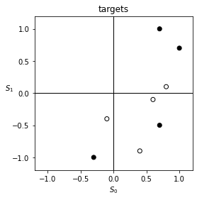
Let us test our network on a classification problem. We will classify points on a 2-d plane into 2 classes. In this case, the input is a 2-d vector, and the output is a 1-d binary number. Here are some sample points with their target labels shown as color.
input_array = np.array([[0.7, 1.],
                        [1., 0.7],
                        [0.7, -0.5],
                        [-0.3, -1.],
                        [0.4, -0.9],
                        [-0.1, -0.4],
                        [0.6, -0.1],
                        [0.8, 0.1]])    # input patterns
target_array = np.array([[1],
                         [1],
                         [1],
                         [1],
                         [-1],
                         [-1],
                         [-1],
                         [-1]])    # target patterns
M = len(input_array)    # number of patterns
plt.figure(figsize=(4,4))
plt.scatter(input_array[:,0], input_array[:,1], c=target_array[:,0], ec='k', cmap='Greys')
plt.axvline(0, color='k', lw=1)
plt.axhline(0, color='k', lw=1)
plt.xlim(-1.2, 1.2)
plt.ylim(-1.2, 1.2)
plt.xlabel(r'$S_0$')
plt.ylabel(r'$S_1$', rotation=0)
plt.title('targets')
plt.show()

Since the points above are not linearly separable, we expect that a simple perceptron will not be able to classify them correctly. Let us first verify this by creating a simple perceptron to try the task.
Ni = input_array.shape[1]    # size of input layer
No = target_array.shape[1]    # size of output layer
net = SimplePerceptron(Ni, No)    # create simple perceptron network

T = 200    # training time
seq = np.random.randint(M, size=T)    # random sequences of input patterns

for s in seq:
    net.train(input_array[s], target_array[s])    # train network by presenting input-output pairs
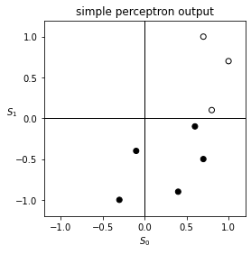
After training, we will make the network calculate the output for each input pattern. We will plot the points, colored according to the output, and see if they are classified correctly.
output_array = []
for inp in input_array:
    out = net.run(inp).copy()    # make a copy so that it will not be overwritten
    output_array.append(out)
output_array = np.asarray(output_array)
plt.figure(figsize=(4,4))
plt.scatter(input_array[:,0], input_array[:,1], c=output_array[:,0], ec='k', cmap='Greys')
plt.axvline(0, color='k', lw=1)
plt.axhline(0, color='k', lw=1)
plt.xlim(-1.2, 1.2)
plt.ylim(-1.2, 1.2)
plt.xlabel(r'$S_0$')
plt.ylabel(r'$S_1$', rotation=0)
plt.title('simple perceptron output')
plt.show()

As expected, the simple perceptron cannot do it. Notice that the points are segregated by color, because the decision boundary of a simple perceptron is a straight line.
Now let us try a multi-layer perceptron to see if it has superior performance. We will use a single, large hidden layer, say 10 times the size of the input layer.
Ni = input_array.shape[1]    # size of input layer
Nh = 10*Ni    # size of hidden layer
No = target_array.shape[1]    # size of output layer
net = MultilayerPerceptron([Ni, Nh, No])    # create network

T = 1000    # training time
seq = np.random.randint(M, size=T)    # random sequence of indices for input patterns

for s in seq:
    net.train(input_array[s], target_array[s], learning_rate=0.01)    # train network by presenting input-output pairs
Notice that we have chosen a small learning rate. If the learning rate is too large, the network might jump around the parameter space and not converge. On the other hand, if the learning rate is too small, it might take a long time for the network to converge to a solution. Finding an appropriate learning rate is one aspect of training networks that requires experience.
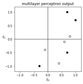
Let us check if this multi-layer perceptron classifies the points correctly.
output_array = []
for inp in input_array:
    out = net.run(inp).copy()    # make a copy so that it will not be overwritten
    output_array.append(out)
output_array = np.asarray(output_array)
plt.figure(figsize=(4,4))
plt.scatter(input_array[:,0], input_array[:,1], c=output_array[:,0], ec='k', cmap='Greys')
plt.axvline(0, color='k', lw=1)
plt.axhline(0, color='k', lw=1)
plt.xlim(-1.2, 1.2)
plt.ylim(-1.2, 1.2)
plt.xlabel(r'$S_0$')
plt.ylabel(r'$S_1$', rotation=0)
plt.title('multilayer perceptron output')
plt.show()

You may see that the outputs agree with the desired targets. (If not, try training the network again, since one might get unlucky.) This demonstrates that a multi-layer network with hidden layers is much more powerful than a single-layer network.

