Coupled Oscillators

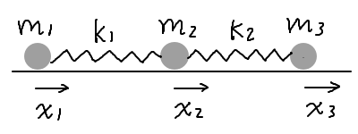
Consider three masses connected by two springs, moving freely along a horizontal line. The masses are \(m_1\), \(m_2\), and \(m_3\), and the spring constants are \(k_1\) and \(k_2\). Let \(x_1\), \(x_2\), and \(x_3\) be the displacements of the masses from an equilibrium position, such that the springs are relaxed when \(x_1 = x_2 = x_3 = 0\). We would like to solve the equations of motion for the displacements \(x_i\), \(i = 1, 2, 3\).

The Lagrangian of the system is given by:

(22)\[\begin{equation} L = \frac12 m_1 \dot{x}_1^2 + \frac12 m_2 \dot{x}_2^2 + \frac12 m_3 \dot{x}_3^2 - \frac12 k_1 (x_2 - x_1)^2 - \frac12 k_2 (x_3 - x_2)^2 \end{equation}\]

The Euler-Lagrange equations for \(x_i\) are:

(23)\[\begin{align} m_1 \ddot{x}_1 &= - k_1 (x_1 - x_2) \\ m_2 \ddot{x}_2 &= - k_1 (x_2 - x_1) - k_2 (x_2 - x_3) \\ m_3 \ddot{x}_3 &= - k_2 (x_3 - x_2) \\ \end{align}\]

These can be written in a matrix form as:

(24)\[\begin{equation} \left( \begin{array}{c} \ddot{x}_1 \\ \ddot{x}_2 \\ \ddot{x}_3 \end{array} \right) = - \left( \begin{array}{ccc} k_1 / m_1 & - k_1 / m_1 & 0 \\ - k_1 / m_2 & (k_1 + k_2) / m_2 & - k_2 / m_2 \\ 0 & - k_2 / m_3 & k_2 / m_3 \end{array} \right) \cdot \left( \begin{array}{c} x_1 \\ x_2 \\ x_3 \end{array} \right) \end{equation}\]

or simply

(25)\[\begin{equation} \ddot{\mathbf{X}} = - \mathbf{A} \cdot \mathbf{X} \end{equation}\]

where the vector \(\mathbf{X} \equiv (x_1, x_2, x_3)^\top\) is what we want to solve for as a function of time. For simplicity, we assume that the initial velocities are zero, \(\dot{x}_i(0) = 0\), so we only need to specify the initial displacements \(x_i(0)\).

Brute-force numerical solution

We can of course solve the coupled ODEs directly, using the scipy.integrate.odeint function as we did before. Here is the code for doing that. Note that we have to define velocities \(v_i \equiv \dot{x}_i\) as auxiliary variables in order to turn the equations to first-order.

import numpy as np
np.set_printoptions(suppress=True)
import scipy.integrate as intgr
import matplotlib.pyplot as plt

def equations(X, t, m1, m2, m3, k1, k2):
    x1, x2, x3, v1, v2, v3 = X    # unpack variables
    dx1 = v1
    dx2 = v2
    dx3 = v3
    dv1 = -k1/m1 * x1 + k1/m1 * x2
    dv2 = k1/m2 * x1 - (k1+k2)/m2 * x2 + k2/m2 * x3
    dv3 = k2/m3 * x2 - k2/m3 * x3
    dXdt = [dx1, dx2, dx3, dv1, dv2, dv3]    # pack derivatives
    return dXdt

# choose parameters
m1, m2, m3 = 1, 2, 3
k1, k2 = 2, 1

# specify initial values
x1i, x2i, x3i = 0, 0.4, -0.4
v1i, v2i, v3i = 0, 0, 0
init = [x1i, x2i, x3i, v1i, v2i, v3i]

T = 20.    # total time to solve for
time = np.arange(0, T, 0.1)    # time points to evaluate solution at

sol = intgr.odeint(equations, init, time, args=(m1, m2, m3, k1, k2))    # solve equations
X = sol[:,0:3]    # vector X consists of the first three components of the solution

plt.figure()
for i in range(3):
    plt.plot(time, X[:,i], label=f'$x_{i+1}$')
plt.ylim(-1, 1)
plt.xlabel(r'$t$')
plt.ylabel(r'$x_i$')
plt.legend(ncol=3)
plt.show()

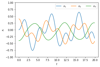
The dynamics look a bit “chaotic”. To gain more insight into the dynamics, we will decompose them into normal modes using matrix diagonalization.

Normal modes

Suppose \(\mathbf{A}\) can be diagonalized as:

(26)\[\begin{equation} \mathbf{A} = \mathbf{R} \cdot \mathbf{D} \cdot \mathbf{R}^{-1} \end{equation}\]

where \(\mathbf{D}\) is a diagonal matrix formed by the eigenvalues of \(\mathbf{A}\), and \(\mathbf{R}\) is a matrix whose columns are the corresponding eigenvectors of \(\mathbf{A}\), i.e.,

(27)\[\begin{equation} \mathbf{D} = \left( \begin{array}{ccc} \lambda_1 & & \\ & \lambda_2 & \\ & & \lambda_3 \end{array} \right) \,, \qquad \mathbf{R} = \left( \begin{array}{ccc} & & \\ \vec{\xi^{(1)}} & \vec{\xi^{(2)}} & \vec{\xi^{(3)}} \\ & & \end{array} \right) \end{equation}\]

We can use \(\mathbf{R}\) to transform \(\mathbf{X}\) to a new set of variables \(\mathbf{X}' \equiv \mathbf{R}^{-1} \cdot \mathbf{X}\). With this transformation, the equation for \(\mathbf{X}'\) simplifies to:

(28)\[\begin{equation} \ddot{\mathbf{X}'} = - \mathbf{D} \cdot \mathbf{X}' \end{equation}\]

Thus, each component satisfies an equation \(\ddot{x}'_i = - \lambda_i x'_i\), the solution of which is just:

(29)\[\begin{equation} x'_i(t) = x'_i(0) \cos(\omega_i t) \end{equation}\]

with \(\mathbf{X}'(0) = \mathbf{R}^{-1} \cdot \mathbf{X}(0)\) and \(\omega_i = \sqrt{\lambda_i}\) (we need \(\lambda_i \geq 0\), which is true for \(\mathbf{A}\), as shown below). Therefore, the solution for the original variables can be written as a sum over normal modes:

(30)\[\begin{equation} \mathbf{X}(t) = \mathbf{R} \cdot \mathbf{X}'(t) = \sum_i \vec{\xi^{(i)}} x'_i(0) \cos(\omega_i t) \end{equation}\]

Each mode has its own frequency of oscillation \(\omega_i\), and the normalized eigenvector \(\vec{\xi^{(i)}}\) represents the “direction” of each mode, whereas \(x'_i(0)\) represents the “amplitude” of each mode.

To construct the solution using the normal modes as described above, let us first find the eigenvalues and eigenvectors of the matrix \(\mathbf{A}\). This can be done using the numpy.linalg.eig function. Note that \(\mathbf{A}\) will be symmetric only if all masses are equal, in which case we can use numpy.linalg.eigh instead.

A = np.array([[k1/m1, -k1/m1, 0],
              [-k1/m2, (k1+k2)/m2, -k2/m2],
              [0, -k2/m3, k2/m3]])

D, R = np.linalg.eig(A)    # calculate eigenvalues and eigenvectors
print(f'eigenvalues = {D}')    # each entry `D[i]` is an eigenvalue
print(f'eigenvectors = \n{R}')    # each column `R[:,i]` is the corresponding eigenvector
# D = np.around(D, 8)    # remove truncation error if necessary

eigenvalues = [3.21034789 0.62298544 0.        ]
eigenvectors = 
[[ 0.85399876  0.6897631   0.57735027]
 [-0.5168178   0.47490692  0.57735027]
 [ 0.05987895 -0.54652565  0.57735027]]

Note that all eigenvalues are non-negative (barring truncation error, which can be removed by uncommenting the last line of code). From these we can obtain the frequencies of the normal modes and their amplitudes.

freq = np.sqrt(D)    # each entry is a normal frequency
amp = np.dot(np.linalg.inv(R), [x1i, x2i, x3i])    # each entry is the corresponding amplitude

Then we can sum over the normal modes to obtain the solution.

modes = np.zeros((3, len(time)))    # to construct normal modes
for i in range(3):
    modes[i,:] = amp[i] * np.cos(freq[i] * time)    # each normal mode as a function of time
X_sum = np.dot(R, modes)

Let us compare the solutions we constructed using normal modes to those found above by brute-force.

plt.figure()
for i in range(3):
    plt.plot(time, X[:,i], label=f'$x_{i+1}$')    # solutions found by brute-force
    plt.plot(time, X_sum[i,:], 'k:')    # solutions found using normal modes
plt.ylim(-1, 1)
plt.xlabel(r'$t$')
plt.ylabel(r'$x_i$')
plt.legend(ncol=3)
plt.show()

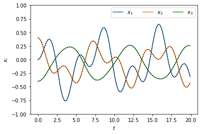
As expected, the solutions lie perfectly on top of each other.

Decomposing the motion

To better visualize the motion, we can decompose it into superposition of the normal modes. We will plot these modes in separate figures below.

fig, ax = plt.subplots(1,3, figsize=(18,4))
for n in range(3):    # plot each mode
    for i in range(3):    # for each mode, plot all variables x_i
        x_i = R[i,n] * modes[n,:]
        ax[n].plot(time, x_i, label=f'$x_{i+1}$')
    ax[n].set_ylim(-1, 1)
    ax[n].set_xlabel(r'$t$')
    ax[n].set_ylabel(r'$x_i$')
    ax[n].legend(ncol=3)
    ax[n].set_title(f'mode {n+1}: $\omega_{n+1} = {freq[n]:.3f}$')
plt.show()

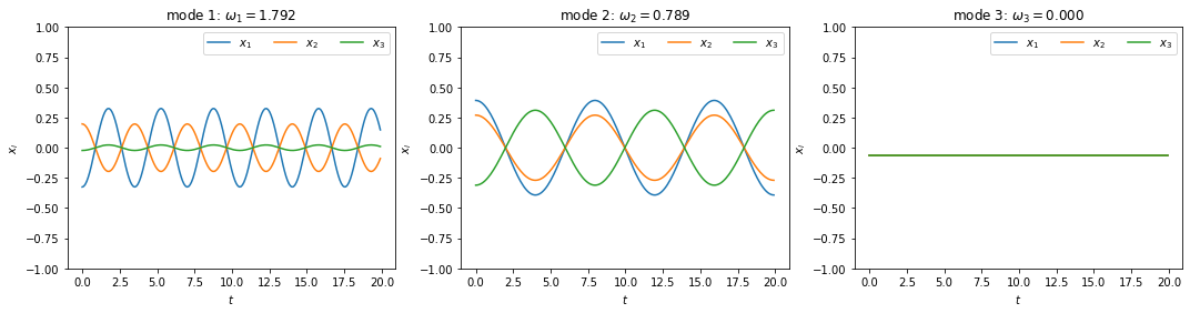
It can be seen that the three modes oscillate at different frequencies — actually, the third mode has a zero frequency, meaning that it does not oscillate at all! That is because this mode represents the motion of the center of mass, which is not moving since there is no external force and the initial velocity is zero. For each of the other modes, the three variables oscillate at the same frequency but with different amplitudes, and they can be in or out of phase with one another.

We can make an animation to visualize these modes and their superposition as below.

import matplotlib.animation as anim

plt.rcParams["animation.html"] = "jshtml"
fig, ax = plt.subplots(figsize=(4,4))
ax.set_xlim(-1, 3)
ax.set_ylim(-0.5, 3.5)
ax.axis('off')
ax.text(-1, 0.2, 'all modes')
ax.text(-1, 1.2, 'mode 1')
ax.text(-1, 2.2, 'mode 2')
ax.text(-1, 3.2, 'mode 3')
p1, = ax.plot([], [], 'o-')    # plot masses in mode 1
p2, = ax.plot([], [], 'o-')    # plot masses in mode 2
p3, = ax.plot([], [], 'o-')    # plot masses in mode 3
p0, = ax.plot([], [], 'o-')    # plot masses in all modes
offset = np.arange(3)    # add natural length of springs

def animate(t):
    p1.set_data(R[:,0]*modes[0,t] + offset, [1, 1, 1])
    p2.set_data(R[:,1]*modes[1,t] + offset, [2, 2, 2])
    p3.set_data(R[:,2]*modes[2,t] + offset, [3, 3, 3])
    p0.set_data(X_sum[:,t] + offset, [0, 0, 0])

mov = anim.FuncAnimation(fig, animate, frames=len(time), interval=50)
plt.close()

mov

Once Loop Reflect

Finally, we can plot the configuration of the system in a 3-D \((x_1, x_2, x_3)\) space to visualize the superposition of the modes.

fig3D = plt.figure(figsize=(8,8))
ax = fig3D.add_subplot(projection='3d')
ax.set_xlim(-1, 1)
ax.set_ylim(-1, 1)
ax.set_zlim(-1, 1)
ax.set_xlabel(f'$x_1$')
ax.set_ylabel(f'$x_2$')
ax.set_zlabel(f'$x_3$')
ax.plot3D([R[0,0], -R[0,0]], [R[1,0], -R[1,0]], [R[2,0], -R[2,0]], 'blue')    # plot eigenvector 1
ax.plot3D([R[0,1], -R[0,1]], [R[1,1], -R[1,1]], [R[2,1], -R[2,1]], 'orange')    # plot eigenvector 2
ax.plot3D([R[0,2], -R[0,2]], [R[1,2], -R[1,2]], [R[2,2], -R[2,2]], 'green')    # plot eigenvector 3
p1, = ax.plot3D([], [], [], 'o')    # plot displacements in mode 1
p2, = ax.plot3D([], [], [], 'o')    # plot displacements in mode 2
p3, = ax.plot3D([], [], [], 'o')    # plot displacements in mode 3
p0, = ax.plot3D([], [], [], '-')    # plot displacements in all modes

def animate3D(t):
    p1.set_data([R[0,0]*modes[0,t]], [R[1,0]*modes[0,t]])
    p1.set_3d_properties([R[2,0]*modes[0,t]])
    p2.set_data([R[0,1]*modes[1,t]], [R[1,1]*modes[1,t]])
    p2.set_3d_properties([R[2,1]*modes[1,t]])
    p3.set_data([R[0,2]*modes[2,t]], [R[1,2]*modes[2,t]])
    p3.set_3d_properties([R[2,2]*modes[2,t]])
    p0.set_data(X_sum[0,:t+1], X_sum[1,:t+1])
    p0.set_3d_properties(X_sum[2,:t+1])
    ax.view_init(azim=30+t)
    
mov3D = anim.FuncAnimation(fig3D, animate3D, frames=len(time), interval=50)
plt.close()

mov3D

Once Loop Reflect

In this plot, the lines represent the directions of the eigenvectors, and the dots represent the instantaneous values of the normal modes, which oscillate along the corresponding directions with different frequencies. We have also plotted the trajectory of the overall configuration of the system, which is the vector sum of the normal modes at every instant. This plot shows that the eigenvectors provide a new set of basis vectors in the configuration space, and the normal modes are the components of the system configuration along these bases. The matrix diagonalization that we did can be thought of as a change of basis in the configuration space, such that the oscillations are decoupled. Note that, if the matrix is symmetric, then the eigenvectors are orthogonal to each other; otherwise, the new basis vectors are non-orthogonal, and the normal modes as the components along these directions are not simple projections of the total displacement (but are projections along the dual bases which are the left eigenvectors of the matrix).