Numerical Integration of a Function

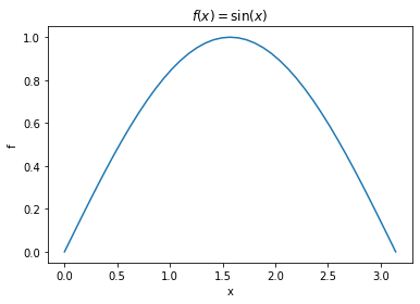
Suppose we have a function \(f(x)\) that we want to integrate. For example, \(f(x) = \sin(x)\), to be integrated from \(0\) to \(\pi\). The result should be

\[\begin{equation*} \int_{0}^{\pi} \sin(x) dx = - \cos(x) \Big|_{0}^{\pi} = 2 \end{equation*}\]

But how about we evaluate the integral numerically?

import numpy as np
import matplotlib.pyplot as plt

Let us first define the function to be integrated and plot it.

def func(x):
    f = np.sin(x)    # use the `sin` function from numpy
    return f

N = 40    # number of partitions used below
x_array = np.linspace(0, np.pi, N+1)    # this function uniformly partitions a range and returns an array (endpoint included)
f_array = func(x_array)    # apply our function on the array (element-wise)

plt.figure()
plt.plot(x_array, f_array)
plt.xlabel('x')
plt.ylabel('f')
plt.title(r'$f(x) = \sin (x)$')
plt.show()

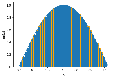
Integration using Riemann Sum

The integral of the function is the area under the curve. We can integrate the function by partitioning the x-axis into small segments and approximating the area within each partition as a rectangle. Then the total area is approximated by the sum of all rectangle areas.

dx = np.pi / N

plt.figure()
plt.plot(x_array, f_array)
plt.bar(x_array, f_array, width=dx, edgecolor='orange')    # make bar plot
plt.xlabel('x')
plt.ylabel('sin(x)')
plt.show()

Riemann_sum = np.sum(f_array * dx)
print(f'Total area = {Riemann_sum}')

Total area = 1.998971810497066

If we increase the number of partitions, N, we can improve the precision of the numerical integration. To do this, let us define a function that carries out the steps we did above, but with N as a parameter.

def sum_over_N_part(N):
    """
    integrate a function using Riemann sum over N partitions.
    input:
    N: int, number of partitions.
    output:
    Riemann_sum: float, value of integral.
    """
    x_array = np.linspace(0, np.pi, N+1)
    f_array = func(x_array)    # note that `func` has been defined outside this function
    dx = np.pi / N
    Riemann_sum = np.sum(f_array * dx)
    return Riemann_sum

First check if we can reproduce our result above:

sum_over_N_part(40)

1.998971810497066

Now let us try a bigger N:

sum_over_N_part(100)

1.9998355038874436

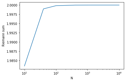
In fact, we can see how our result improves by plotting the result with respect to N:

N_array = [10, 40, 100, 400, 1000, 4000, 10000]    # try these N values
sum_array = []
for N in N_array:
    s = sum_over_N_part(N)
    sum_array.append(s)

plt.figure()
plt.plot(N_array, sum_array)
plt.xscale('log')    # use `log` scale
plt.xlabel('N')
plt.ylabel('Riemann sum')
plt.show()

Let us check how fast the numerical result converges to the right answer:

err_array = np.abs(2 - np.array(sum_array))    # absolute deviation from the right answer

plt.figure()
plt.plot(N_array, err_array)
plt.xscale('log')
plt.yscale('log')
plt.xlabel('N')
plt.ylabel('error')
plt.show()

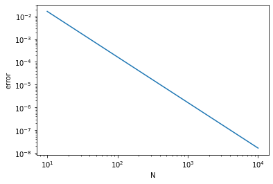
This figure shows that the numerical result converges to the right answer quadratically, i.e., error \(\propto N^{-2}\).

Integration using Monte Carlo

An alternative, perhaps amusing, method for doing the integral is to use the “Monte Carlo” method. Monte Carlo generally refers to numerical methods that rely on using (pseudo)random numbers. In our case, we will generate random numbers to help us estimate the area under the curve.

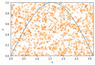
The idea is to look at a box that contains the curve, such as one bounded by \(x = 0, \pi\) and \(y = 0, 1\). Our goal is to estimate the fraction of area inside the box that is under the curve. Since we know the total area of the box, \(A = \pi\), by evaluating the fraction, we will be able to find the area under the curve. Now the trick is to estimate this fraction using random numbers. Basically, we will toss random points inside the box and count how many happen to lie below the curve.

R = 1000    # number of random points

y_coord = np.random.rand(R)    # y coordinates uniformly sampled between 0 and 1
x_coord = np.random.rand(R) * np.pi    # x coordinates uniformly sampled between 0 and pi

plt.figure()
plt.plot(x_array, f_array)    # plotting the curve
plt.plot(x_coord, y_coord, 'x')    # plotting the random points
plt.xlim(0, np.pi)
plt.ylim(0, 1)
plt.xlabel('x')
plt.ylabel('y')
plt.show()

below_curve = (y_coord < func(x_coord))    # binary array, 1 for True (below curve) and 0 for False (above curve)
count_below = np.sum(below_curve)    # count the number of points below the curve
print(f'number of points below the curve = {count_below}')

number of points below the curve = 650

fraction = count_below / R    # fraction of points below the curve
MonteCarlo_area = np.pi * fraction    # estimated area below the curve
print(f'Area under curve = {MonteCarlo_area}')

Area under curve = 2.0420352248333655

We may improve the precision by increasing the number of random points, R. Let us again define a function to carry out the steps above, with the number R as a parameter:

def estimate_by_R_points(R):
    """
    Define a python function to do the integral using R random points.
    Input:
    R: int, number of random points.
    Output:
    MonteCarlo_area: float, value of integral as given by Monte Carlo method.
    """
    y_coord = np.random.rand(R)
    x_coord = np.random.rand(R) * np.pi
    below_curve = (y_coord < func(x_coord))
    count_below = np.sum(below_curve)
    fraction = count_below / R
    MonteCarlo_area = np.pi * fraction
    return MonteCarlo_area

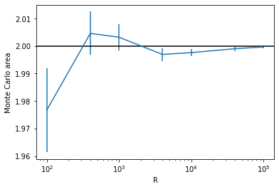
Let us plot the result with respect to the number R. Since each time we run the function, there will be a different realization of the random points, we should take an average over multiple trials for each R. We will also estimate the error of the estimation by calculating the standard error among the trials.

R_array = [100, 400, 1000, 4000, 10000, 40000, 100000]    # try these R values
est_array = []    # list of estimates
se_array = []    # list of standard errors

trial = 100
for R in R_array:
    res = []
    for t in range(trial):    # for each R, repeat the calculation `trial` times
        mc = estimate_by_R_points(R)
        res.append(mc)    # collect results from the trials in the list `res`
    res_mean = np.mean(res)    # calculate the mean of the trials
    res_se = np.std(res) / np.sqrt(trial)    # standard error = standard deviation / sqrt(#data-points)
    est_array.append(res_mean)
    se_array.append(res_se)

plt.figure()
plt.errorbar(R_array, est_array, yerr=se_array)    # make plot with errorbars
plt.axhline(2, color='k')    # draw horizontal line
plt.xscale('log')
plt.xlabel('R')
plt.ylabel('Monte Carlo area')
plt.show()

Now we can see how the error scales with the number of random points:

plt.figure()
plt.plot(R_array, se_array)
plt.xscale('log')
plt.yscale('log')
plt.xlabel('R')
plt.ylabel('standard error')
plt.show()

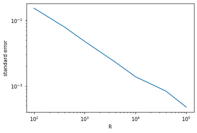
This figure shows that our result converges again quadratically, i.e., error \(\propto R^{-2}\).