Numerical Solution of Ordinary Differential Equations (ODE)

In this chapter, we will learn to numerically solve a set of ODEs. To do so, we will use the odeint function from the scipy.integrate package.

import numpy as np
import matplotlib.pyplot as plt
import scipy.integrate as intgr

Suppose the equations we want to solve are:

\[\begin{align*} \dot{X}_1 &= f_1(X_1, X_2, \cdots) \\ \dot{X}_2 &= f_2(X_1, X_2, \cdots) \\ &\;\vdots \end{align*}\]

Note that if your equations are higher-order, you need to first convert them to first order ODEs by introducing auxiliary variables.

As an example, let us consider the Lotka-Volterra system with two variables:

\[\begin{align*} \dot{X} &= r X - f X Y \\ \dot{Y} &= g X Y - d Y \end{align*}\]

These equations describe the population dynamics of a predator and a prey species (see more details in Lotka-Volterra System).

First, we need to define a function that calculates the time derivatives, i.e., the right-hand side of the equations.

def equations(x, t, r, f, g, d):
    """
    inputs:
    x: array, all variables stacked into an array.
    t: float, time (need to have the argument `t` even if the equations do not depend on time explicitly).
    r, f, g, d: other parameters used in the equations.
    """
    X, Y = x    # parse variables
    dXdt = r * X - f * X * Y
    dYdt = g * X * Y - d * Y
    return [dXdt, dYdt]    # assemble derivatives into an array

Now we can integrate our differential equations using odeint. We specify a set of time points at which we would like to know the values of the variables. Then we ask the function odeint to return these values at the given time points.

r = 5    # growth rate of the prey
f = r    # feeding rate of the predator
g = 1    # growth rate of the predator per prey available
d = 1    # death rate of the predator

T = 10.    # total time to solve the equations for
time = np.arange(0, T, 0.01)    # time points to evaluate the solutions at
X0, Y0 = np.random.rand(2)    # random initial values between 0 and 1

sol = intgr.odeint(equations, [X0, Y0], time, args=(r,f,g,d))    # solve ODE

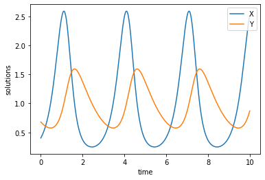
The solution is an array of shape (\(n_t\), \(n_v\)), where the first axis is the number of time points, and the second axis is the number of variables. We can now plot these solutions:

Xt = sol[:,0]
Yt = sol[:,1]

plt.figure()
plt.plot(time, Xt, label='X')
plt.plot(time, Yt, label='Y')
plt.xlabel('time')
plt.ylabel('solutions')
plt.legend(loc='upper right')
plt.show()

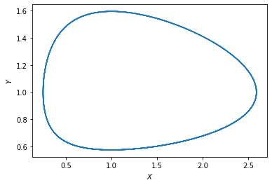
Or in phase space (in this case, the solution is a closed orbit):

plt.figure()
plt.plot(Xt, Yt)
plt.xlabel(r'$X$')
plt.ylabel(r'$Y$')
plt.show()